Show code
from pathlib import Path
import sys
import matplotlib
import matplotlib.pyplot as plt
import numpy as np
import pandas as pd
import seaborn as snsA hands-on exercise for designing clear, accurate, accessible, and purposeful data visualizations with Python
Hands-on exercises and step-by-step tools for doing, applying, and building evidence.
A hands-on exercise for designing clear, accurate, accessible, and purposeful data visualizations with Python
This CDI Practical is designed to be completed actively rather than read passively. You will transform a cleaned service-delivery dataset into a small, coherent visual evidence package.
Work through the practical in order. For each chart, begin with a question and audience, create a first version, critique it, and improve it. Run every code block and inspect both the chart and the data supporting it.
You are encouraged to:
Follow the rendered HTML practical in a browser while working in VS Code. Use VS Code to run, adapt, and save the Python workflow. JupyterLab, Positron, or Google Colab can also be used, but the repository paths and final Quarto render are designed for VS Code.
Complete the practical in four passes.
Identify the audience, decision, question, variables, and necessary context before creating a chart.
Select charts for comparison, distribution, relationship, composition, or change over time. Build accurate first versions from verified summaries.
Improve hierarchy, labels, ordering, colour, accessibility, annotations, and consistency. Test whether the main message remains clear without narration.
Export a coordinated visual evidence package, document design decisions and limitations, render the HTML, and review it in a browser.
Data visualization is not the final decorative step of analysis. It is a reasoning and communication process. A chart selects, transforms, encodes, and emphasizes information; each choice can clarify evidence or distort it.
This practical continues from Data Science Practicals 001 and 002. You will use the cleaned service-delivery dataset and the exploratory questions developed during EDA, then create visualizations intended for an analytical briefing.
The workflow uses Python with pandas, numpy, matplotlib, and seaborn. No optional statistical or visualization dependencies are required.
By completing this practical, you will be able to:
By the end of the practical, you will create:
Suggested output structure:
results/
├── figures/
│   ├── records-by-region.png
│   ├── age-distribution.png
│   ├── age-and-satisfaction.png
│   ├── service-mix-by-region.png
│   ├── monthly-service-volume.png
│   ├── annotated-follow-up-chart.png
│   ├── satisfaction-small-multiples.png
│   └── visual-summary.png
└── tables/
    ├── visualization-plan.csv
    ├── chart-data-region.csv
    ├── chart-data-monthly.csv
    ├── chart-data-service-mix.csv
    ├── chart-data-follow-up.csv
└── visualization-decision-log.csvYou need Python 3.10 or later, VS Code with the Python and Jupyter extensions, Quarto, and a dedicated project environment.
From the repository root, create and activate .venv.
macOS or Linux
python3 -m venv .venv
source .venv/bin/activate
Windows PowerShell
py -m venv .venv
.venv\Scripts\Activate.ps1
Install the required packages into the activated environment:
python -m pip install --upgrade pip
python -m pip install -r requirements.txt
Verify that the terminal is using the project environment and that the core packages import successfully:
python --version
python -c "import pandas, numpy, matplotlib, seaborn; print('Visualization environment ready')"
In VS Code, choose Python: Select Interpreter from the Command Palette and select the Python interpreter inside .venv. Manual Jupyter-kernel registration is not required. When you return to the project later, reactivate .venv before running Python or quarto render.
The practical uses:
data/cleaned-service-data.csvKeep the input unchanged. All derived tables and figures belong under results/.
data-visualization-practical/
├── .gitignore
├── AGENTS.md
├── LICENSE
├── README.md
├── requirements.txt
├── practical-before-split.qmd
├── assets/css/
├── data/
│   └── cleaned-service-data.csv
├── results/
│   ├── figures/
│   └── tables/
├── scripts/bash/
│   └── split-practical.sh
├── scripts/python/
├── _quarto.yml
└── practical.qmd              # created during the later split stage
Open the repository root in VS Code so relative paths work consistently.
The supplied cleaned dataset is the learner’s starting point. The completed results/ files are reference outputs for comparison; regenerate your own outputs while completing the guided steps. Any Python utility later placed under scripts/python/ is an optional author/reviewer reproducibility aid, not a replacement for the step-by-step learner workflow. Such a script must resolve the repository root with Path(__file__).resolve().parents[2], read inputs only from top-level data/, and write outputs only to top-level results/.
One row represents one fictional service record. The analytical variables include region, service type, age, visit date, satisfaction score, follow-up requirement, and a retained review flag.
Direct identifiers are not needed for this practical. In real projects, remove names and contact details from visualization workflows unless they are essential and appropriately protected.
The visual communication scenario is:
A programme team needs a concise briefing on service reach, service mix, participant characteristics, satisfaction, follow-up needs, and changes in service volume over time.
Before choosing charts, complete this statement:
For [audience], this visual evidence package will explain [question or pattern] so they can [interpretation, discussion, or decision], while recognizing [important limitation].
For the example practical:
from pathlib import Path
import sys

import matplotlib
import matplotlib.pyplot as plt
import numpy as np
import pandas as pd
import seaborn as snspd.set_option("display.max_columns", 20)
sns.set_theme(style="whitegrid", context="notebook")
CDI_GREEN = "#2F6B4F"
CDI_GOLD = "#D7A84B"
CDI_BLUE = "#4878A8"
CDI_RED = "#B55245"
CDI_GREY = "#6B7280"
plt.rcParams.update(
{
"figure.dpi": 110,
"savefig.dpi": 300,
"axes.titleweight": "bold",
"axes.titlesize": 13,
"axes.labelsize": 10,
"legend.frameon": False,
}
)DATA_PATH = Path("data/cleaned-service-data.csv")
RESULTS_DIR = Path("results")
FIGURES_DIR = RESULTS_DIR / "figures"
TABLES_DIR = RESULTS_DIR / "tables"
for directory in [FIGURES_DIR, TABLES_DIR]:
directory.mkdir(parents=True, exist_ok=True)pd.Series(
{
"python": sys.version.split()[0],
"pandas": pd.__version__,
"numpy": np.__version__,
"matplotlib": matplotlib.__version__,
"seaborn": sns.__version__,
},
name="version",
)python 3.12.6
pandas 2.3.3
numpy 2.1.3
matplotlib 3.10.0
seaborn 0.13.2
Name: version, dtype: objectif not DATA_PATH.exists():
raise FileNotFoundError(f"Expected input file: {DATA_PATH}")
source_data = pd.read_csv(DATA_PATH)
df = source_data.copy()
required_columns = {
"record_id", "region", "service_type", "age", "visit_date",
"satisfaction_score", "follow_up_required", "requires_review"
}
missing_columns = sorted(required_columns.difference(df.columns))
assert not missing_columns, f"Missing required columns: {missing_columns}"
df["visit_date"] = pd.to_datetime(df["visit_date"], errors="coerce")
df["age"] = pd.to_numeric(df["age"], errors="coerce")
df["satisfaction_score"] = pd.to_numeric(df["satisfaction_score"], errors="coerce")
df.head()| record_id | participant_name | region | service_type | age | visit_date | satisfaction_score | follow_up_required | contact_email | requires_review | |
|---|---|---|---|---|---|---|---|---|---|---|
| 0 | SR-0001 | Synthetic Participant 001 | North | Outreach | 40.0 | 2025-08-09 | 4.0 | No | synthetic001@example.invalid | No |
| 1 | SR-0002 | Synthetic Participant 002 | East | Consultation | 48.0 | 2025-11-04 | 4.0 | No | synthetic002@example.invalid | No |
| 2 | SR-0003 | Synthetic Participant 003 | Central | Diagnostics | 40.0 | 2025-09-14 | 4.0 | No | synthetic003@example.invalid | No |
| 3 | SR-0004 | Synthetic Participant 004 | East | Training | NaN | 2025-05-07 | 4.0 | No | synthetic004@example.invalid | No |
| 4 | SR-0005 | Synthetic Participant 005 | West | Consultation | 28.0 | 2025-12-30 | 4.0 | No | synthetic005@example.invalid | No |
pd.Series(
    {
        "records": len(df),
        "variables": df.shape[1],
        "missing_record_ids": int(df["record_id"].isna().sum()),
        "duplicate_non_missing_record_ids": int(
            df.loc[df["record_id"].notna(), "record_id"].duplicated().sum()
        ),
        "records_requiring_review": int(df["requires_review"].astype(str).str.lower().eq("true").sum()),
        "first_visit": df["visit_date"].min(),
        "last_visit": df["visit_date"].max(),
    },
    name="value",
)
records 240
variables 10
missing_record_ids 0
duplicate_non_missing_record_ids 0
records_requiring_review 0
first_visit 2025-01-01 00:00:00
last_visit 2025-12-31 00:00:00
Name: value, dtype: objectservice_types = sorted(df["service_type"].dropna().unique())
service_colours = sns.color_palette("colorblind", n_colors=len(service_types))
SERVICE_PALETTE = dict(zip(service_types, service_colours))
SERVICE_PALETTE{'Consultation': (0.00392156862745098,
0.45098039215686275,
0.6980392156862745),
'Diagnostics': (0.8705882352941177, 0.5607843137254902, 0.0196078431372549),
'Outreach': (0.00784313725490196, 0.6196078431372549, 0.45098039215686275),
'Training': (0.8352941176470589, 0.3686274509803922, 0.0)}Use this same colour mapping whenever service type appears in more than one chart. The colourblind-friendly palette reduces avoidable ambiguity, while labels and position continue to carry the essential meaning.
Identifier issues retained from the cleaning practical do not prevent aggregate charts, but they must remain visible in the quality record. Do not use the number of unique identifiers as a participant count until those records are resolved.
Create a plan connecting each question to a visual task, chart, encoding, audience need, and caution.
visualization_plan = pd.DataFrame(
    [
        ["Where are records concentrated?", "comparison", "ordered bar", "length and position", "Counts are not coverage rates"],
        ["What is the age distribution?", "distribution", "histogram", "position and area", "Missing age values are excluded"],
        ["How do age and satisfaction relate?", "relationship", "scatter plot", "x-y position", "Association is not causation"],
        ["How does service mix differ by region?", "composition", "100% stacked bar", "length and colour", "Small groups can look unstable"],
        ["How does service volume change over time?", "time", "line chart", "x-y position", "Partial months require caution"],
        ["Where is follow-up workload concentrated?", "comparison", "annotated bar", "length and annotation", "Records may not equal unique people"],
    ],
    columns=["question", "task", "chart", "primary_encoding", "caution"],
)
visualization_plan| question | task | chart | primary_encoding | caution | |
|---|---|---|---|---|---|
| 0 | Where are records concentrated? | comparison | ordered bar | length and position | Counts are not coverage rates |
| 1 | What is the age distribution? | distribution | histogram | position and area | Missing age values are excluded |
| 2 | How do age and satisfaction relate? | relationship | scatter plot | x-y position | Association is not causation |
| 3 | How does service mix differ by region? | composition | 100% stacked bar | length and colour | Small groups can look unstable |
| 4 | How does service volume change over time? | time | line chart | x-y position | Partial months require caution |
| 5 | Where is follow-up workload concentrated? | comparison | annotated bar | length and annotation | Records may not equal unique people |
visualization_plan.to_csv(TABLES_DIR / "visualization-plan.csv", index=False)Prefer encodings people compare accurately:
Use bar charts for precise category comparisons, lines for ordered time, points for relationships, and histograms or box plots for distributions. Pie charts, three-dimensional effects, and decorative pictograms often make comparison harder.
Two analysts can use the same chart type and communicate different ideas through the denominator, ordering, scale, grouping, annotations, and title. Record these decisions explicitly.
Prepare the chart data separately so its values can be checked and exported.
region_counts = (
    df["region"]
    .value_counts()
    .sort_values(ascending=True)
    .rename_axis("region")
    .reset_index(name="records")
)
region_counts.to_csv(TABLES_DIR / "chart-data-region.csv", index=False)
region_counts| region | records | |
|---|---|---|
| 0 | West | 49 |
| 1 | North | 51 |
| 2 | East | 68 |
| 3 | Central | 72 |
fig, ax = plt.subplots(figsize=(9, 5))
bars = ax.barh(region_counts["region"], region_counts["records"], color=CDI_GREEN)
ax.bar_label(bars, padding=4, fontsize=9)
ax.set(
    title="Service records are unevenly distributed across regions",
    xlabel="Number of service records",
    ylabel="",
)
ax.spines[["top", "right", "left"]].set_visible(False)
ax.grid(axis="y", visible=False)
ax.set_xlim(0, region_counts["records"].max() * 1.15)
fig.tight_layout()
fig.savefig(FIGURES_DIR / "records-by-region.png", bbox_inches="tight")
plt.show()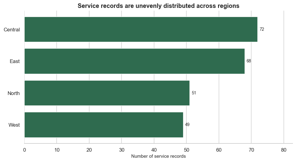
The zero baseline preserves proportional comparison. Ordering reduces search effort, and direct labels remove the need to estimate values from gridlines.
valid_age = df["age"].dropna()
median_age = valid_age.median()

fig, ax = plt.subplots(figsize=(9, 5))
sns.histplot(valid_age, bins=12, color=CDI_BLUE, edgecolor="white", ax=ax)
ax.axvline(median_age, color=CDI_RED, linewidth=2, linestyle="--",
           label=f"Median: {median_age:.0f} years")
ax.set(
    title="Participant ages span a broad range",
    xlabel="Age (years)",
    ylabel="Number of records",
)
ax.legend()
fig.tight_layout()
fig.savefig(FIGURES_DIR / "age-distribution.png", bbox_inches="tight")
plt.show()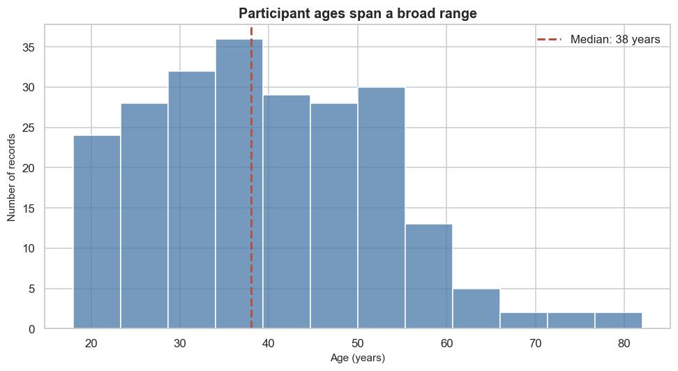
State that missing ages are excluded and report the valid sample size. Bin width affects perceived shape, so check nearby choices rather than searching for the most dramatic result.
Satisfaction is an ordinal, bounded score. Plot individual observations without adding an optional statistical smoother or implying a continuous outcome.
relationship_data = df[["age", "satisfaction_score", "service_type"]].dropna()

fig, ax = plt.subplots(figsize=(9, 5.5))
sns.scatterplot(
    data=relationship_data,
    x="age",
    y="satisfaction_score",
    hue="service_type",
    palette=SERVICE_PALETTE,
    alpha=0.65,
    s=55,
    ax=ax,
)
ax.set(
    title="Age and satisfaction show substantial overlap",
    xlabel="Age (years)",
    ylabel="Satisfaction score",
    yticks=range(1, 6),
)
ax.legend(title="Service type", bbox_to_anchor=(1.02, 1), loc="upper left")
fig.tight_layout()
fig.savefig(FIGURES_DIR / "age-and-satisfaction.png", bbox_inches="tight")
plt.show()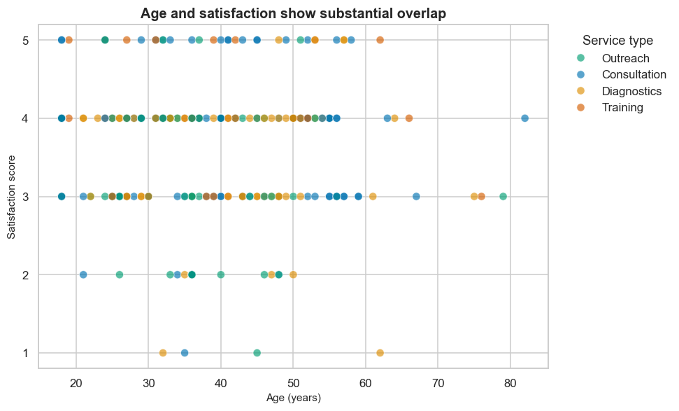
Colour adds a third variable, so use it only when the service groups help answer the question. Overlap, missing pairs, and the limited score range constrain interpretation.
Use a 100% stacked bar when the question is about service mix within regions rather than regional volume.
service_mix = pd.crosstab(df["region"], df["service_type"], normalize="index").mul(100)
service_mix.rename_axis(columns="service_type").to_csv(
    TABLES_DIR / "chart-data-service-mix.csv"
)
service_mix.round(1)| service_type | Consultation | Diagnostics | Outreach | Training |
|---|---|---|---|---|
| region | ||||
| Central | 36.1 | 22.2 | 26.4 | 15.3 |
| East | 33.8 | 25.0 | 23.5 | 17.6 |
| North | 39.2 | 15.7 | 27.5 | 17.6 |
| West | 30.6 | 38.8 | 22.4 | 8.2 |
fig, ax = plt.subplots(figsize=(10, 5.5))
service_mix.plot(
    kind="barh",
    stacked=True,
    color=[SERVICE_PALETTE[column] for column in service_mix.columns],
    width=0.72,
    ax=ax,
)
ax.set(
    title="Service mix varies across regions",
    xlabel="Share of regional service records (%)",
    ylabel="",
    xlim=(0, 100),
)
ax.legend(title="Service type", bbox_to_anchor=(1.02, 1), loc="upper left")
fig.tight_layout()
fig.savefig(FIGURES_DIR / "service-mix-by-region.png", bbox_inches="tight")
plt.show()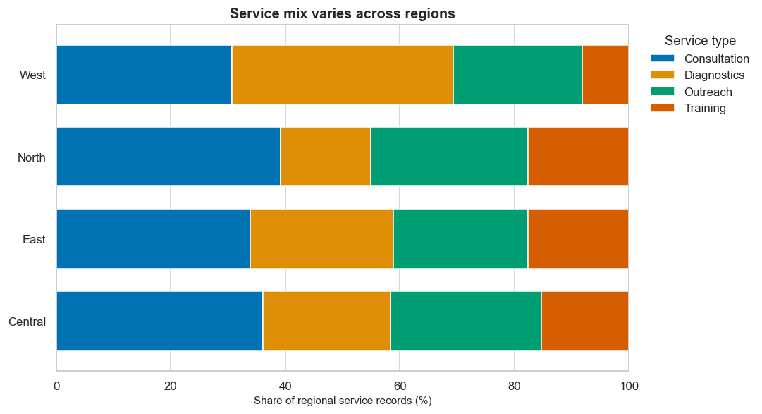
Only the first and last segments share a common baseline. If precise comparison of every service type is important, use small multiple bars instead.
monthly_volume = (
    df.dropna(subset=["visit_date"])
    .assign(month=lambda x: x["visit_date"].dt.to_period("M").dt.to_timestamp())
    .groupby("month")
    .size()
    .rename("records")
    .reset_index()
    .sort_values("month")
)
monthly_volume.to_csv(TABLES_DIR / "chart-data-monthly.csv", index=False)
monthly_volume| month | records | |
|---|---|---|
| 0 | 2025-01-01 | 29 |
| 1 | 2025-02-01 | 16 |
| 2 | 2025-03-01 | 15 |
| 3 | 2025-04-01 | 21 |
| 4 | 2025-05-01 | 21 |
| 5 | 2025-06-01 | 25 |
| 6 | 2025-07-01 | 17 |
| 7 | 2025-08-01 | 19 |
| 8 | 2025-09-01 | 14 |
| 9 | 2025-10-01 | 24 |
| 10 | 2025-11-01 | 21 |
| 11 | 2025-12-01 | 18 |
expected_months = pd.date_range(
    monthly_volume["month"].min(),
    monthly_volume["month"].max(),
    freq="MS",
)
missing_months = expected_months.difference(monthly_volume["month"])

pd.Series(
    {
        "observed_months": len(monthly_volume),
        "missing_months": len(missing_months),
        "first_month_records": int(monthly_volume.iloc[0]["records"]),
        "last_month_records": int(monthly_volume.iloc[-1]["records"]),
    },
    name="value",
)
observed_months 12
missing_months 0
first_month_records 29
last_month_records 18
Name: value, dtype: int64If missing_months is greater than zero, do not silently connect the gap. Reindex to the full sequence only when domain knowledge supports treating an unobserved month as zero; otherwise leave the gap visible and explain it.
fig, ax = plt.subplots(figsize=(11, 5))
ax.plot(monthly_volume["month"], monthly_volume["records"],
        color=CDI_GREEN, marker="o", linewidth=2.2)
ax.set(
    title="Monthly service volume fluctuates across the observation period",
    xlabel="Visit month",
    ylabel="Number of service records",
)
ax.spines[["top", "right"]].set_visible(False)
ax.grid(axis="x", visible=False)
fig.autofmt_xdate(rotation=30)
fig.tight_layout()
fig.savefig(FIGURES_DIR / "monthly-service-volume.png", bbox_inches="tight")
plt.show()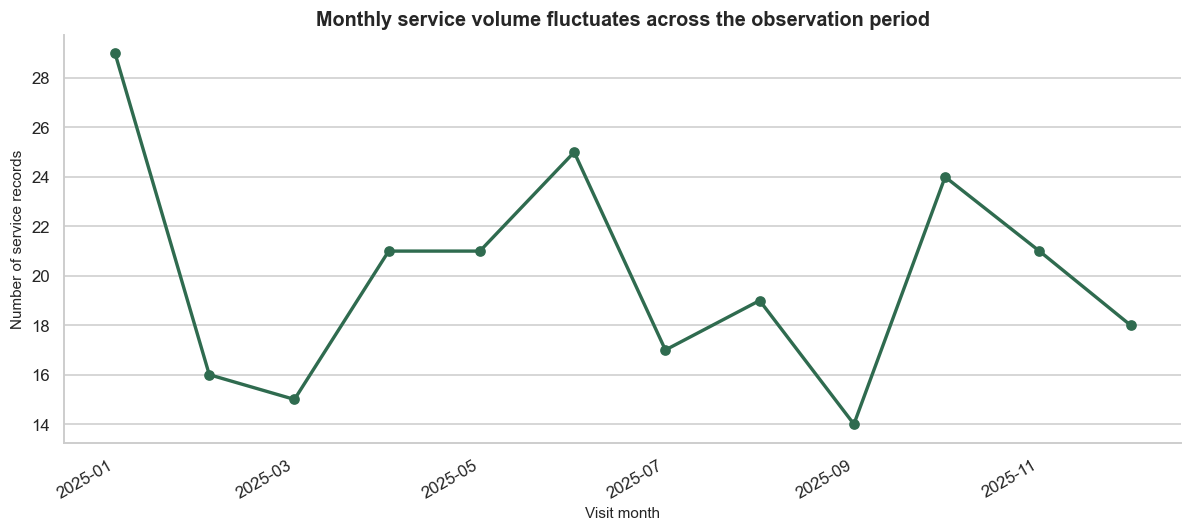
Time must be continuous. Check for missing months and partial first or last periods before interpreting rises and falls.
Colour can identify categories, order intensity, or highlight a focus. It should not carry essential information alone.
The CDI palette used here is restrained, but accessibility still depends on context, contrast, size, and redundant encoding.
A descriptive title states the subject. A message title states the main evidence. Use message titles only when the evidence is strong enough and the wording does not overclaim.
follow_up_by_region = (
    df.assign(
        needs_follow_up=(
            df["follow_up_required"].astype("string").str.strip().str.casefold().eq("yes")
        )
    )
    .groupby("region", as_index=False)
    .agg(records=("record_id", "size"), follow_up_records=("needs_follow_up", "sum"))
)
follow_up_by_region["follow_up_percent"] = (
    follow_up_by_region["follow_up_records"].div(follow_up_by_region["records"]).mul(100)
)
follow_up_by_region = follow_up_by_region.sort_values("follow_up_percent")
follow_up_by_region.to_csv(TABLES_DIR / "chart-data-follow-up.csv", index=False)
follow_up_by_region| region | records | follow_up_records | follow_up_percent | |
|---|---|---|---|---|
| 2 | North | 51 | 6 | 11.764706 |
| 3 | West | 49 | 12 | 24.489796 |
| 1 | East | 68 | 17 | 25.0 |
| 0 | Central | 72 | 19 | 26.388889 |
fig, ax = plt.subplots(figsize=(9, 5))
bars = ax.barh(
    follow_up_by_region["region"],
    follow_up_by_region["follow_up_percent"],
    color=[CDI_GREY] * (len(follow_up_by_region) - 1) + [CDI_GOLD],
)
ax.bar_label(bars, labels=[f"{value:.1f}%" for value in follow_up_by_region["follow_up_percent"]],
             padding=4, fontsize=9)
ax.set(
    title="Follow-up requirements are concentrated differently by region",
    xlabel="Records requiring follow-up (%)",
    ylabel="",
)
ax.set_xlim(0, max(50, follow_up_by_region["follow_up_percent"].max() * 1.2))
ax.spines[["top", "right", "left"]].set_visible(False)
ax.grid(axis="y", visible=False)
fig.tight_layout()
fig.savefig(FIGURES_DIR / "annotated-follow-up-chart.png", bbox_inches="tight")
plt.show()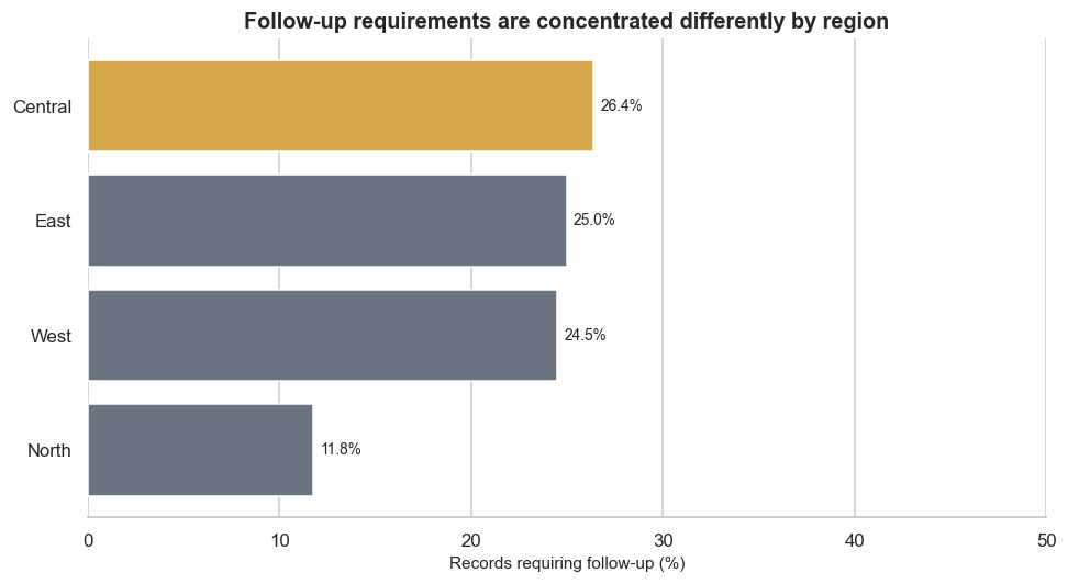
The highlighted bar directs attention, but the title remains cautious. The percentage denominator is all records within each region.
Small multiples repeat the same visual scale across groups, making patterns easier to compare than a crowded chart.
grid = sns.catplot(
    data=df,
    x="satisfaction_score",
    col="service_type",
    col_wrap=2,
    kind="count",
    order=range(1, 6),
    color=CDI_GREEN,
    height=3.3,
    aspect=1.25,
    sharey=True,
)
grid.set_axis_labels("Satisfaction score", "Number of records")
grid.set_titles("{col_name}")
grid.figure.suptitle("Satisfaction distributions by service type", y=1.03, fontweight="bold")
grid.figure.savefig(FIGURES_DIR / "satisfaction-small-multiples.png", bbox_inches="tight")
plt.show()
Shared axes support comparison. If group sizes differ substantially, add sample sizes or use percentages depending on the question.
Use this review sequence for every visual:
Do not crop a bar chart axis to exaggerate differences, delete valid observations to make a pattern cleaner, use area to encode a one-dimensional value, or select only the time period that supports a preferred story.
Combine a small number of complementary views. A visual summary should have one purpose and a clear reading order.
fig, axes = plt.subplots(2, 2, figsize=(13, 10))

axes[0, 0].barh(region_counts["region"], region_counts["records"], color=CDI_GREEN)
axes[0, 0].set(title="Service records by region", xlabel="Records", ylabel="")

sns.histplot(df["age"].dropna(), bins=12, color=CDI_BLUE, edgecolor="white", ax=axes[0, 1])
axes[0, 1].set(title="Participant age distribution", xlabel="Age (years)", ylabel="Records")

axes[1, 0].plot(monthly_volume["month"], monthly_volume["records"],
                color=CDI_GREEN, marker="o", linewidth=2)
axes[1, 0].set(title="Monthly service volume", xlabel="Visit month", ylabel="Records")
axes[1, 0].tick_params(axis="x", rotation=30)

axes[1, 1].barh(follow_up_by_region["region"], follow_up_by_region["follow_up_percent"],
                color=CDI_GOLD)
axes[1, 1].set(title="Follow-up requirement by region", xlabel="Records requiring follow-up (%)", ylabel="")

for ax in axes.flat:
    ax.spines[["top", "right"]].set_visible(False)

fig.suptitle("Service-delivery visual summary", fontsize=17, fontweight="bold", y=1.01)
fig.tight_layout()
fig.savefig(FIGURES_DIR / "visual-summary.png", bbox_inches="tight")
plt.show()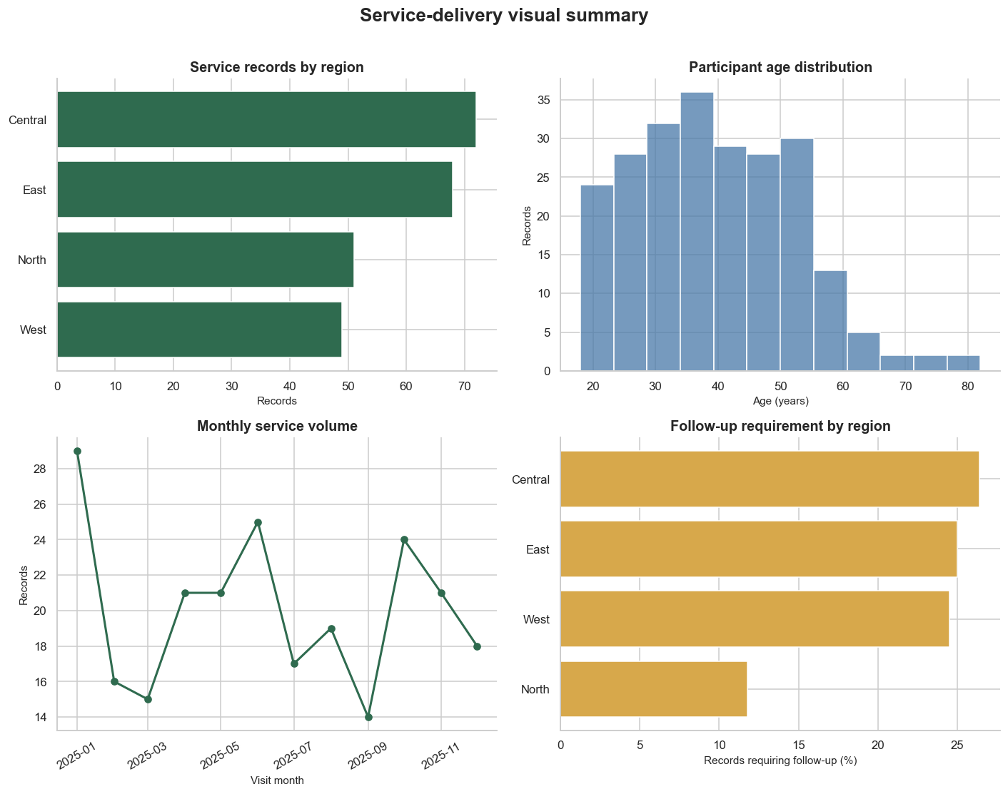
Provide a short text summary beside the figure in any published product. Alternative text should describe the chart’s purpose and main pattern, not every pixel or design element.
A chart that works on a large monitor may fail in a report, slide, phone, or printed page.
Check each final figure at:
Increase text size, simplify legends, or separate panels when a reduced chart becomes difficult to read. Never rely on hover text for essential meaning in a static deliverable.
decision_log = pd.DataFrame(
    [
        ["records by region", "ordered horizontal bar", "accurate category comparison and readable labels", "counts do not measure population coverage"],
        ["age distribution", "histogram with median", "shows shape while locating a robust centre", "bin choice changes perceived shape"],
        ["age and satisfaction", "scatter plot", "shows overlap and individual observations", "ordinal scores and overplotting limit precision"],
        ["service mix", "100% stacked bar", "compares within-region composition", "middle segments lack a shared baseline"],
        ["monthly volume", "line chart", "uses ordered time and preserves continuity", "partial months may be incomplete"],
        ["follow-up by region", "highlighted horizontal bar", "shows percentages with explicit labels", "regional record counts differ"],
    ],
    columns=["visual", "design_choice", "reason", "limitation"],
)
decision_log| visual | design_choice | reason | limitation | |
|---|---|---|---|---|
| 0 | records by region | ordered horizontal bar | accurate category comparison and readable labels | counts do not measure population coverage |
| 1 | age distribution | histogram with median | shows shape while locating a robust centre | bin choice changes perceived shape |
| 2 | age and satisfaction | scatter plot | shows overlap and individual observations | ordinal scores and overplotting limit precision |
| 3 | service mix | 100% stacked bar | compares within-region composition | middle segments lack a shared baseline |
| 4 | monthly volume | line chart | uses ordered time and preserves continuity | partial months may be incomplete |
| 5 | follow-up by region | highlighted horizontal bar | shows percentages with explicit labels | regional record counts differ |
decision_log.to_csv(TABLES_DIR / "visualization-decision-log.csv", index=False)Write one concise paragraph describing the visual evidence package and one paragraph defining its limits. Address:
Use phrases such as “the records show,” “within this dataset,” and “the visual comparison suggests.” Do not claim that a service, region, or participant characteristic caused an outcome.
expected_outputs = [
    TABLES_DIR / "visualization-plan.csv",
    TABLES_DIR / "chart-data-region.csv",
    TABLES_DIR / "chart-data-monthly.csv",
    TABLES_DIR / "chart-data-service-mix.csv",
    TABLES_DIR / "chart-data-follow-up.csv",
    TABLES_DIR / "visualization-decision-log.csv",
    FIGURES_DIR / "records-by-region.png",
    FIGURES_DIR / "age-distribution.png",
    FIGURES_DIR / "age-and-satisfaction.png",
    FIGURES_DIR / "service-mix-by-region.png",
    FIGURES_DIR / "monthly-service-volume.png",
    FIGURES_DIR / "annotated-follow-up-chart.png",
    FIGURES_DIR / "satisfaction-small-multiples.png",
    FIGURES_DIR / "visual-summary.png",
]

output_check = pd.DataFrame(
    {"path": [str(path) for path in expected_outputs], "exists": [path.exists() for path in expected_outputs]}
)
assert output_check["exists"].all(), "One or more expected outputs were not created."
output_check| path | exists | |
|---|---|---|
| 0 | results/tables/visualization-plan.csv | True |
| 1 | results/tables/chart-data-region.csv | True |
| 2 | results/tables/chart-data-monthly.csv | True |
| 3 | results/tables/chart-data-service-mix.csv | True |
| 4 | results/tables/chart-data-follow-up.csv | True |
| 5 | results/tables/visualization-decision-log.csv | True |
| 6 | results/figures/records-by-region.png | True |
| 7 | results/figures/age-distribution.png | True |
| 8 | results/figures/age-and-satisfaction.png | True |
| 9 | results/figures/service-mix-by-region.png | True |
| 10 | results/figures/monthly-service-volume.png | True |
| 11 | results/figures/annotated-follow-up-chart.png | True |
| 12 | results/figures/satisfaction-small-multiples.png | True |
| 13 | results/figures/visual-summary.png | True |
Render from the VS Code terminal:
source .venv/bin/activate  # macOS or Linux
quarto render
On Windows PowerShell, activate with .venv\Scripts\Activate.ps1 before rendering.
Open products/index.html in a browser. Check navigation, layout, figure size, labels, code blocks, text contrast, mobile resizing, and whether the visual message remains clear.
Your portfolio evidence should include:
Use this portfolio framing:
How can service-delivery records be visualized clearly and responsibly to communicate differences in service reach, participant characteristics, satisfaction, follow-up needs, service mix, and activity over time?
Revise it when working with another dataset. A useful visualization question includes an audience and purpose, not only variables.
Describe what one row represents, the analysis period, the number of records, the variables visualized, remaining missingness, privacy considerations, and the limits of the dataset’s coverage.
Do not publish real direct identifiers. Visualizations can reveal sensitive information even when names are absent, especially for small groups or precise locations.
Summarize the project as a reproducible sequence:
Choose one visualization that best serves the intended audience. Present it with a clear title, a short evidence statement, a denominator or sample-size note, a limitation, and the action or question it should prompt.
Document that:
Explain how data limitations and design choices affect interpretation. Note what a chart leaves out, which comparison is easiest or hardest, and what additional data would support a stronger conclusion.
List only tools used in the completed project. The standard workflow uses Python, pandas, numpy, matplotlib, seaborn, VS Code, Quarto, and optionally Git and GitHub for version control and sharing.
Write brief responses to these prompts:
The next practical can build from this visual evidence into a focused statistical or modelling workflow.
Before marking the practical complete, confirm that you have:
You have completed Data Science Practical 003: Data Visualization Practical.
You now have a reproducible visual communication workflow, a coordinated set of figures and supporting tables, and portfolio evidence demonstrating that you can make deliberate choices about audience, chart form, scale, colour, annotation, accessibility, and interpretation.
Keep the cleaned source, complete practical.qmd, exported results, and rendered HTML together. They provide a traceable record from data to visual message and a reusable foundation for future analytical communication.