A hands-on exercise for investigating distributions, relationships, outliers, and patterns in a cleaned dataset with Python
Author
Complex Data Insights
Published
Aug 2026
COMPLEX DATA INSIGHTS
CDI Practicals
Hands-on exercises and step-by-step tools for doing, applying, and building evidence.
Exploratory Data Analysis Practical
A hands-on exercise for investigating distributions, relationships, outliers, and patterns in a cleaned dataset with Python
AuthorComplex Data Insights
PublishedAug 2026
ID CDI-DATASCIENCE-PRACTICAL-002
Type Practical Product
Audience Students, researchers, analysts, professionals, mentors, and learners developing practical data science skills
Theme Responsible exploratory analysis turns a cleaned dataset into questions, patterns, evidence, and clearly stated limitations
How to Use This Practical
This CDI Practical is designed to be completed actively rather than read passively. You will investigate a cleaned service-delivery dataset and build a reproducible exploratory data analysis (EDA) that moves from orientation to interpretation.
Work through the practical in order. Run each code block, inspect its output, and write short observations before moving on. Keep unusual values visible until you have evidence that they are errors. Exploratory findings are signals for further investigation, not proof of causes.
You are encouraged to:
begin with explicit exploratory questions;
connect each table or plot to a question;
examine missing values and outliers without automatically removing them;
distinguish description, interpretation, and explanation;
preserve the cleaned input dataset;
record limitations and possible next analyses;
adapt the workflow to a dataset relevant to your own work.
Browser-first workflow
This practical is delivered as an online HTML page. Keep the practical open beside VS Code, work through it in order, and run or adapt each Python code block in your own environment. You may also use JupyterLab, Positron, Google Colab, or another environment that supports Python notebooks or scripts.
Practical Overview
Exploratory data analysis is the disciplined process of learning what a dataset can—and cannot—show before formal modelling or decision-making. It combines questions, summaries, visualizations, checks, and careful interpretation.
In this practical, one row represents one service record. You will examine who used services, where and when services were delivered, how satisfaction varied, which records remain incomplete, and which observations deserve review.
The workflow uses Python with pandas, numpy, matplotlib, and seaborn. It follows four linked stages:
orient yourself to the dataset and define questions;
explore individual variables and missingness;
examine group differences, relationships, and outliers;
communicate findings, uncertainty, and limitations.
Learning Outcomes
By completing this practical, you will be able to:
formulate useful exploratory questions;
confirm that a cleaned dataset is ready for analysis;
distinguish numerical, categorical, date, identifier, and text variables;
produce reproducible descriptive summaries and visualizations;
investigate missingness and potential outliers;
compare groups and examine relationships between variables;
avoid causal claims that the design cannot support;
You need Python 3.10 or later and VS Code with the Python and Jupyter extensions. Run the commands below from the repository root to create a dedicated virtual environment for this practical.
Create the Virtual Environment
python3-m venv .venv
Activate the Virtual Environment
On macOS or Linux:
source .venv/bin/activate
On Windows PowerShell:
.venv\Scripts\Activate.ps1
After activation, your terminal prompt should begin with (.venv).
When you return to the project later, activate .venv again before running any commands. To leave the environment, run deactivate.
The input for this practical is:
data/cleaned-service-data.csv
The project includes a deterministic generator for this synthetic input. You do not need Practical 001 to complete this product. If you use your own cleaned output from Practical 001, confirm that the column names and meanings match before running the code.
Step 1: Confirm the Starting Dataset
Begin inside the extracted project folder. The supplied project files already include:
data/cleaned-service-data.csv
Confirm that the file exists, then preview it without editing the source:
Show code
from pathlib import Pathimport pandas as pdpreview_path = Path("data/cleaned-service-data.csv")assert preview_path.exists(), "Confirm that data/cleaned-service-data.csv is present."pd.read_csv(preview_path).head()
record_id
participant_name
region
service_type
age
visit_date
satisfaction_score
follow_up_required
contact_email
requires_review
0
SR-0001
Synthetic Participant 001
North
Outreach
40.0
2025-08-09
4.0
No
synthetic001@example.invalid
No
1
SR-0002
Synthetic Participant 002
East
Consultation
48.0
2025-11-04
4.0
No
synthetic002@example.invalid
No
2
SR-0003
Synthetic Participant 003
Central
Diagnostics
40.0
2025-09-14
4.0
No
synthetic003@example.invalid
No
3
SR-0004
Synthetic Participant 004
East
Training
NaN
2025-05-07
4.0
No
synthetic004@example.invalid
No
4
SR-0005
Synthetic Participant 005
West
Consultation
28.0
2025-12-30
4.0
No
synthetic005@example.invalid
No
The project also includes a deterministic generator that can recreate the synthetic starting dataset when needed:
python scripts/python/generate-example-dataset.py
The generator uses a fixed random seed to create the same 240 fictional service records. It intentionally retains limited missingness, review flags, unequal groups, and a small number of unusual ages for investigation. Running it is optional and may replace the supplied file, so preserve any dataset you need before using it.
Reference results
The project files include author-generated tables, figures, and quality-control results. Use them to check your progress, but complete the guided analysis yourself so that you understand and can explain every analytical decision.
Step 2: Prepare the Guided Workflow
Open the project folder in VS Code and keep this practical open in your browser. Work through the remaining steps in order, run each code block in your Python environment, inspect its output, and record your own observations. The code will validate the dataset and create an evidence package under results/.
Project Structure
Open the extracted project folder in VS Code. Keep source data in data/ and write your outputs only to results/.
The dataset contains service records with identifiers, participant details, service characteristics, dates, satisfaction scores, follow-up status, and a review flag. Names and email addresses are included only because the dataset is fictional. In real analysis, minimize access to direct identifiers and exclude them from exploratory outputs unless they are essential.
Variable
Role in this analysis
Intended meaning
record_id
Identifier
Unique service record
participant_name
Direct identifier
Fictional participant name
region
Categorical
Service-delivery region
service_type
Categorical
Type of service delivered
age
Numerical
Participant age in years
visit_date
Date
Date of service visit
satisfaction_score
Numerical/ordinal
Rating from 1 to 5
follow_up_required
Categorical/binary
Whether follow-up is required
contact_email
Direct identifier
Fictional contact detail
requires_review
Categorical/binary
Flag retained during cleaning
Define Exploratory Questions
Start with questions rather than charts. This prevents EDA from becoming an unstructured search for anything visually interesting.
Use these core questions:
What does a typical service record look like?
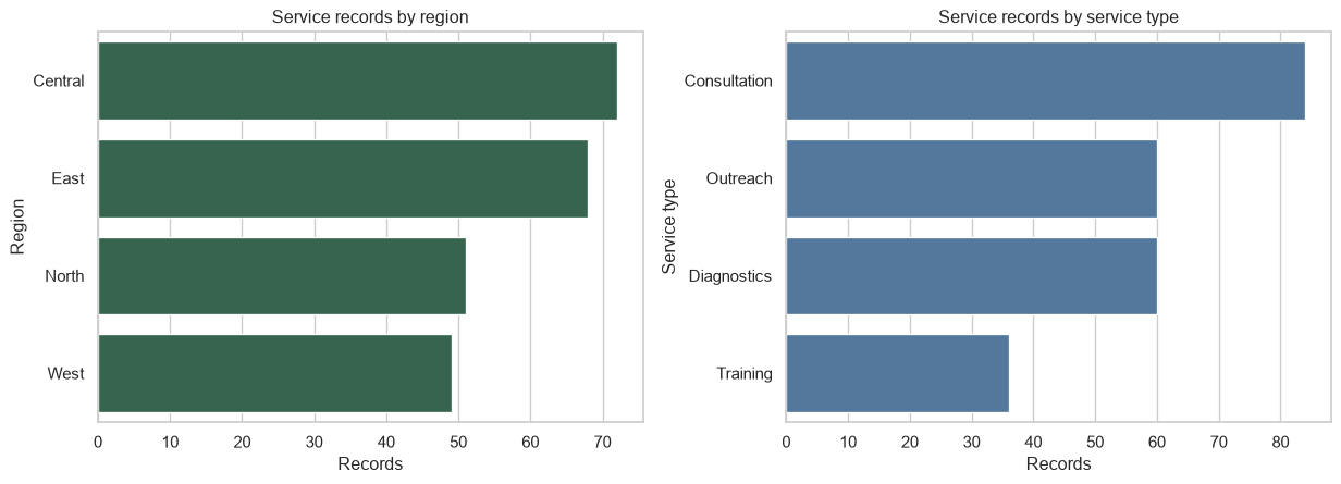
How are records distributed across regions and service types?
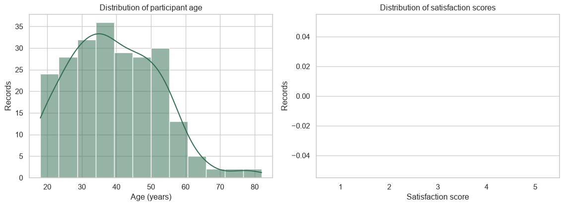
What are the shapes and spreads of age and satisfaction score?
Where does missingness remain, and is it concentrated in particular groups?
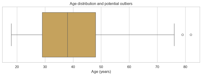
Which observations are potential outliers and what context do they need?
How does satisfaction vary across regions, service types, and follow-up status?
Is age associated with satisfaction in this dataset?
Which patterns are strong enough to motivate a later confirmatory analysis?
Exploratory Analysis Plan
For each question, record:
the question and why it matters;
the variables and unit of analysis;
the summary or visualization you will use;
the expected output;
one interpretation risk or limitation.
Add at least one question of your own before continuing.
Prepare the Analysis Environment
Run the following setup in VS Code as you work through the online practical.
Show code
from pathlib import Pathimport sysimport matplotlibimport matplotlib.pyplot as pltimport numpy as npimport pandas as pdimport seaborn as sns
Load the source once and create an analysis copy. Do not overwrite the input file.
Show code
ifnot DATA_PATH.exists():raiseFileNotFoundError(f"Expected {DATA_PATH}. Run the included generator or place a compatible cleaned dataset in data/." )source_data = pd.read_csv(DATA_PATH)df = source_data.copy()df["visit_date"] = pd.to_datetime(df["visit_date"], errors="coerce")for column in ["age", "satisfaction_score"]: df[column] = pd.to_numeric(df[column], errors="coerce")df.head()
record_id
participant_name
region
service_type
age
visit_date
satisfaction_score
follow_up_required
contact_email
requires_review
0
SR-0001
Synthetic Participant 001
North
Outreach
40.00
2025-08-09
4.00
No
synthetic001@example.invalid
No
1
SR-0002
Synthetic Participant 002
East
Consultation
48.00
2025-11-04
4.00
No
synthetic002@example.invalid
No
2
SR-0003
Synthetic Participant 003
Central
Diagnostics
40.00
2025-09-14
4.00
No
synthetic003@example.invalid
No
3
SR-0004
Synthetic Participant 004
East
Training
NaN
2025-05-07
4.00
No
synthetic004@example.invalid
No
4
SR-0005
Synthetic Participant 005
West
Consultation
28.00
2025-12-30
4.00
No
synthetic005@example.invalid
No
Confirm Analysis Readiness
Cleaning and EDA have different purposes, but EDA still begins with validation. Confirm shape, identifier uniqueness, expected columns, and ranges before interpreting results.
Investigate missing columns, duplicate identifiers, invalid dates, or impossible values before continuing. Do not silently repair the dataset inside the EDA workflow; document the issue and return to the cleaning process when necessary.
Step 4: Profile the Dataset
Understand Variable Types
The same stored type can support different analytical roles. satisfaction_score, for example, is numeric but ordinal: the order is meaningful, while equal spacing between ratings should not be assumed automatically.
Use the overview to identify variables with little variation, unexpected missingness, or a suspicious number of categories. A table is an analytical checkpoint, not merely a required output.
fig, axes = plt.subplots(1, 2, figsize=(13, 4.8))sns.countplot(data=df, y="region", order=df["region"].value_counts().index, color=CDI_GREEN, ax=axes[0])axes[0].set(title="Service records by region", xlabel="Records", ylabel="Region")sns.countplot(data=df, y="service_type", order=df["service_type"].value_counts().index, color=CDI_BLUE, ax=axes[1])axes[1].set(title="Service records by service type", xlabel="Records", ylabel="Service type")fig.tight_layout()fig.savefig(FIGURES_DIR /"categorical-patterns.png", dpi=300, bbox_inches="tight")plt.show()
Counts describe the dataset, not necessarily the population. A region with more records may have more clients, better reporting, a larger service network, or a different sampling process.
Examine Time Coverage and Activity
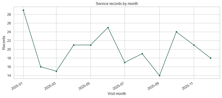
Dates reveal the observation window, gaps, and changes in record volume. They do not by themselves explain why activity changed.
Look for gaps, isolated peaks, and incomplete first or last months. Confirm operational explanations with external context rather than inferring them from the chart alone.
Step 6: Investigate Missingness and Outliers
Investigate Missingness
Missing values can be informative. First locate them, then ask whether they are associated with other observed variables.
Avoid filling missing values simply to make a plot work. Each analysis should state how missing observations were handled and how many records contributed.
Identify and Review Outliers
Use the interquartile-range rule as a screening tool, not a deletion rule.
For every flagged record, ask whether the value is possible, consistent with the source, influential, and relevant to the analysis. A valid extreme value may be one of the most important observations in the dataset.
Step 7: Explore Group Differences and Relationships
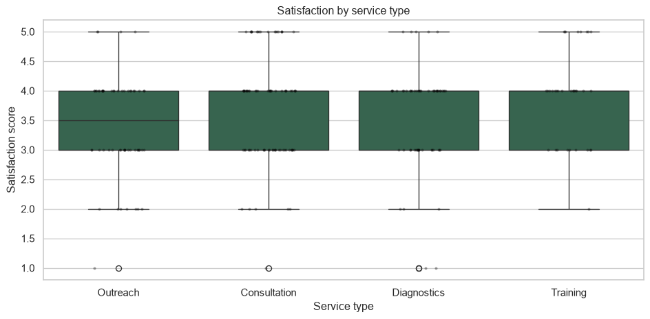
Compare Groups
Group summaries should show sample size as well as centre and spread.
Describe visible differences without claiming that service type caused them. Group composition, case complexity, timing, and selection may also matter.
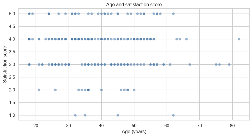
Spearman correlation summarizes monotonic association and suits an ordinal score better than treating it as an unrestricted continuous measure. Still inspect the plot: a single coefficient can hide clusters, non-linearity, and uneven data density.
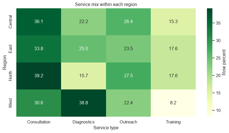
Row percentages answer “within each region, what share of records belongs to each service type?” Counts and percentages answer different questions; keep the denominator explicit.
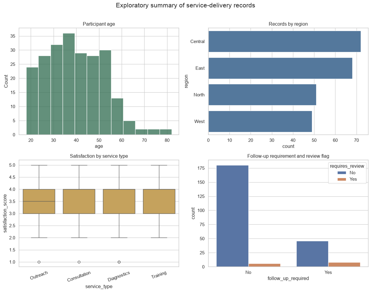
Build an Exploratory Visual Summary
Create one figure that presents the most useful patterns without trying to include every chart.
Check that titles state what is shown, axes and units are labelled, category order is understandable, colours are legible, and the figure can be interpreted without reading the code.
Step 8: Interpret and Communicate the Evidence
Record Key Findings
Create an evidence table that separates observation from interpretation and limitation. Replace the prompts with findings supported by your actual outputs.
Show code
exploratory_findings = pd.DataFrame( [ {"question": "How are records distributed across regions?","evidence": "Complete after inspecting the regional frequency table and chart.","interpretation": "Describe the most and least represented regions.","limitation": "Record counts may reflect service volume or reporting coverage.","next_analysis": "Compare regional coverage with an external population denominator.", }, {"question": "How does satisfaction vary by service type?","evidence": "Complete after inspecting group sizes, medians, spreads, and the grouped plot.","interpretation": "Describe differences without causal language.","limitation": "Scores are ordinal and group composition may differ.","next_analysis": "Use a pre-specified ordinal model with relevant confounders.", }, {"question": "Which observations require further review?","evidence": f"The IQR screen flagged {len(outlier_review)} age value(s).","interpretation": "Flagged values require context; they are not automatically errors.","limitation": "The IQR rule is sensitive to distribution shape and sample size.","next_analysis": "Verify flagged records against source documentation.", }, ])exploratory_findings
Write a concise interpretation that answers the exploratory questions and refers to specific tables or figures. Use measured language such as “the dataset shows,” “records were concentrated,” or “scores tended to differ.” Avoid “proved,” “caused,” or “led to.”
Your limitations statement should address:
the fictional and service-record nature of the data;
whether records represent people, visits, or both;
missing age, satisfaction, or contact information;
any review flags retained after cleaning;
unequal group sizes;
the ordinal and bounded satisfaction scale;
the absence of a population denominator;
multiple patterns explored without confirmatory testing;
inability to infer causality from observational summaries.
Exploration is not confirmation
EDA helps generate and refine questions. If a finding will guide a high-stakes decision, test it with an analysis plan, suitable design, uncertainty estimates, and data collected for that purpose.
Step 9: Verify and Present the Evidence Package
Verify Exported Results
Confirm that the evidence package exists and can be regenerated from the source data.
missing_outputs = output_check.loc[~output_check["exists"], "path"].tolist()assertnot missing_outputs, f"Expected outputs were not created: {missing_outputs}"
Compare your exported files with the supplied author-generated reference results. Small presentation differences may occur across software versions, but the data dimensions, summary values, file set, and analytical conclusions should agree.
Portfolio Evidence
Your portfolio evidence should show both the analytical result and the quality of your reasoning. Include:
a short project title and question;
the cleaned dataset and data dictionary;
the analysis plan;
one dataset overview table;
two or three strong figures rather than every exploratory plot;
a short findings table;
an outlier and missingness decision note;
a reproducible workflow description;
interpretation, limitations, and next steps;
a link to your repository or portfolio presentation when appropriate.
Project Question
Use this portfolio framing:
What patterns in service use, participant characteristics, satisfaction, follow-up requirements, and data completeness can be identified in the cleaned service-delivery dataset, and which patterns warrant further analysis?
Revise the question if you adapt the practical to your own dataset. A good question names the population or records, variables, purpose, and boundaries of the analysis.
Dataset
In your portfolio, describe:
what one row represents;
the number of rows and columns;
the relevant variables and their analytical roles;
where the cleaned dataset came from;
any access, privacy, or ethical constraints;
remaining missingness and review flags.
Do not publish direct identifiers from real data. Replace them with safe identifiers or use aggregated outputs.
Workflow
Summarize the work as a reproducible sequence:
preserved and loaded the cleaned source;
confirmed analysis readiness and variable roles;
created dataset, numerical, and categorical summaries;
examined distributions, missingness, and outliers;
compared groups and variable relationships;
recorded findings separately from interpretations;
exported tables and figures;
documented limitations and next analyses.
Main Result
Select one result that best answers the project question. Present the figure or table with a precise title, one paragraph describing the evidence, and one paragraph explaining why it matters. The main result should be understandable without requiring the reader to inspect every intermediate output.
Quality Checks
State the checks that support confidence in the workflow:
required columns were present;
identifiers and duplicate rows were checked;
dates and numeric fields were parsed explicitly;
valid and missing record counts accompanied summaries;
group sizes were reported;
outliers were reviewed rather than silently deleted;
exported files were verified;
completed outputs were compared with the supplied reference results.
Limitations
Keep limitations specific. Explain how each one affects interpretation and what additional data or analysis would reduce uncertainty. A limitation is not a ceremonial paragraph; it defines the boundary of the evidence.
Tools
List only tools you actually used. For the standard workflow:
Python for reproducible analysis;
pandas and numpy for data summaries;
matplotlib and seaborn for visualization;
VS Code for editing and running the workflow;
Git and GitHub for version control and portfolio sharing, if used.
Step 10: Reflect and Complete the Practical
Reflection and Next Steps
Write brief responses to the following prompts:
Which exploratory question produced the most useful evidence, and why?
Which chart changed or complicated your first interpretation?
How did missingness affect the analyses you could perform?
Which outlier decision required the most judgement?
Where were you most at risk of making a causal claim?
What would you pre-specify before a confirmatory analysis?
How would you adapt this workflow to a larger or more sensitive dataset?
A natural next practical would move from exploration to a focused statistical analysis or predictive modelling workflow, using questions and limitations identified here.
Completion Checklist
Before marking the practical complete, confirm that you have:
Practical Complete
You have completed Data Science Practical 002: Exploratory Data Analysis Practical.
You now have a reproducible EDA workflow, a set of analytical outputs, and portfolio evidence that demonstrates more than chart-making. It shows that you can begin with questions, examine data responsibly, distinguish patterns from proof, and communicate what the evidence can and cannot support.
Keep the starting data, your analysis work, and exported results together. They form a complete record of the analysis and a reusable starting point for future exploratory work.