Statistical Inference Practical

Transform a complex service dataset into clear, defensible, decision-relevant insights

COMPLEX DATA INSIGHTS

CDI Practicals

Hands-on exercises and step-by-step tools for doing, applying, and building evidence.

Statistical Inference Practical

From complex evidence to defensible insight

AuthorComplex Data Insights

PublishedAug 2026

ID: CDI-DATASCIENCE-PRACTICAL-004
Type: Guided end-to-end practical
Audience: Researchers, analysts, postgraduate students, and applied data professionals
Theme: Statistical reasoning, uncertainty, and evidence synthesis

How to Use This Practical

Statistical analysis can feel intimidating because selecting a test is only one part of the work. You must also understand the study design, check assumptions, quantify effects, make a hypothesis decision, and explain what the evidence does—and does not—support.

This practical gives you a repeatable reasoning pattern:

1. Ask a focused research question.
2. Identify the variables and design.
3. State the null and alternative hypotheses.
4. Select and justify the method.
5. check assumptions and data limitations.
6. Run the analysis.
7. report the estimate, uncertainty, statistic, and p-value.
8. assess effect size and practical importance.
9. reject or fail to reject the null hypothesis.
10. translate the evidence into a defensible insight.

We say fail to reject the null hypothesis, not accept the null. A non-significant result does not prove that no effect exists.

The Investigation

A service organization offers three delivery models—Standard, Digital, and Integrated—across four regions. Participants have baseline and follow-up outcome scores, wait times, satisfaction scores, and completion status. Allocation was not randomized.

The central question is:

Which service model produces the strongest outcomes, for whom, and how confidently can we defend that conclusion?

The dataset deliberately contains realistic complexity: repeated measurements, three groups, region effects, correlated outcomes, missing values, unequal sample sizes, continuous and categorical variables, and possible confounding.

Learning Outcomes

By completing the practical, you will be able to:

• distinguish one-sample, independent, paired, and multi-group questions;
• conduct t-tests, one-way ANOVA, Tukey HSD, correlations, and chi-square tests;
• evaluate normality, variance, independence, and expected-count assumptions;
• use Mann–Whitney U, Wilcoxon signed-rank, and Kruskal–Wallis sensitivity analyses;
• report confidence intervals and effect sizes alongside p-values;
• apply Holm correction to a family of tests;
• maintain a hypothesis decision register; and
• synthesize converging and conflicting evidence into a CDI Insight Brief.

What You Will Produce

• a validated analysis dataset with a derived change score;
• descriptive and assumption-check tables;
• seven registered hypothesis tests;
• an ANOVA table and Tukey post-hoc comparisons;
• Pearson and Spearman correlation evidence;
• chi-square observed and expected counts;
• non-parametric sensitivity analyses;
• multiplicity-adjusted decisions;
• four analytical figures;
• a hypothesis decision register; and
• a CDI Insight Brief.

Tools and Requirements

Use Python 3.10 or later, VS Code with the Python and Jupyter extensions, and Quarto. From the repository root, create a dedicated environment:

python3 -m venv .venv
source .venv/bin/activate
python -m pip install --upgrade pip
python -m pip install -r requirements.txt

On Windows PowerShell, activate with .venv\Scripts\Activate.ps1.

Step 1: Generate the Complex Example Dataset

python scripts/python/generate-example-dataset.py

The script creates data/inference-service-data.csv reproducibly. The data are synthetic and contain no real participant records.

Step 2: Run the Reference Workflow

bash scripts/bash/run-workflow.sh

This generates the complete reference evidence package under results/. You will reproduce the reasoning in the guided steps below.

Step 3: Load and Validate the Evidence

from pathlib import Path
import numpy as np
import pandas as pd
from scipy import stats
from statsmodels.stats.multicomp import pairwise_tukeyhsd
from statsmodels.stats.multitest import multipletests
import matplotlib.pyplot as plt
import seaborn as sns

DATA = Path("data/inference-service-data.csv")
ALPHA = 0.05
df = pd.read_csv(DATA, parse_dates=["visit_date"])

required = {
    "participant_id", "region", "service_model", "age",
    "baseline_score", "followup_score", "wait_time_minutes",
    "satisfaction_score", "completed_program", "visit_date"
}
assert not required.difference(df.columns)
assert df["participant_id"].is_unique
df["change_score"] = df["followup_score"] - df["baseline_score"]
df.shape, df.isna().sum()

((360, 11),
 participant_id        0
 region                0
 service_model         0
 age                   6
 baseline_score        0
 followup_score        7
 wait_time_minutes     0
 satisfaction_score    5
 completed_program     0
 visit_date            0
 change_score          7
 dtype: int64)

Interpretation checkpoint: Missingness is part of the evidence. Record which analyses use complete cases, how many observations remain, and whether missing outcomes could bias the conclusion.

Step 4: Translate Questions into an Analysis Plan

ID	Research question	Variables and design	Primary method
H1	Is mean improvement above a meaningful 3-point benchmark?	One change score versus a fixed value	One-sample t-test
H2	Does improvement differ between Integrated and Standard?	Two independent groups	Welch t-test
H3	Did participants improve from baseline to follow-up?	Two measurements on the same people	Paired t-test
H4	Does improvement differ across all three models?	Continuous outcome, three groups	One-way ANOVA + Tukey HSD
H5	Is wait time linearly related to satisfaction?	Two continuous variables	Pearson correlation
H6	Is age monotonically related to satisfaction?	Two ordinal/continuous variables	Spearman correlation
H7	Is completion associated with service model?	Two categorical variables	Chi-square independence test

For every row, the null hypothesis states no difference or association in the target population. The alternative states that a difference or association exists. H1 is directional because the benchmark question was prespecified as greater than.

Step 5: Describe Before You Test

descriptive = df.groupby("service_model", observed=True).agg(
    n=("participant_id", "size"),
    baseline_mean=("baseline_score", "mean"),
    followup_mean=("followup_score", "mean"),
    change_mean=("change_score", "mean"),
    change_sd=("change_score", "std"),
    satisfaction_mean=("satisfaction_score", "mean"),
    wait_mean=("wait_time_minutes", "mean"),
    completion_rate=("completed_program", lambda x: x.eq("Yes").mean()),
).round(3)
descriptive

	n	baseline_mean	followup_mean	change_mean	change_sd	satisfaction_mean	wait_mean	completion_rate
service_model
Digital	116	57.647	63.211	5.480	5.703	3.802	17.922	0.638
Integrated	124	56.634	63.230	6.562	7.082	4.094	24.951	0.677
Standard	120	57.742	59.948	2.044	5.501	3.287	28.580	0.517

sns.set_theme(style="whitegrid")
fig, ax = plt.subplots(figsize=(9, 5.5))
sns.violinplot(data=df, x="service_model", y="change_score", inner=None, color="#b9d8cf", ax=ax)
sns.stripplot(data=df, x="service_model", y="change_score", color="#16324f", alpha=.35, ax=ax)
ax.axhline(3, color="#b22222", linestyle="--", label="3-point benchmark")
ax.set(xlabel="Service model", ylabel="Follow-up minus baseline", title="Improvement varies within and between service models")
ax.legend()
plt.tight_layout()
plt.show()

Figure 1: Participant improvement by service model. The dashed line is the prespecified 3-point meaningful benchmark.

Step 6: Check Assumptions Without Treating Them as Rituals

Method	Important conditions	What to inspect	Sensible response
t-test / ANOVA	Independent observations; approximately normal residuals	Design, distributions, Q-Q plot, influential values	Use robust/non-parametric sensitivity analysis; investigate design problems
Standard ANOVA	Similar group variances	Group spreads; Brown–Forsythe test	Consider Welch ANOVA; report sensitivity
Pearson correlation	Linear relationship without dominant outliers	Scatterplot and residual pattern	Add Spearman; consider transformation or nonlinear method
Chi-square	Independent observations and adequate expected counts	Expected-frequency table	Combine defensible categories or use an exact method

normality = []
for model, group in df.groupby("service_model"):
    statistic, p_value = stats.shapiro(group["change_score"].dropna())
    normality.append({"model": model, "W": statistic, "p_value": p_value})

variance_test = stats.levene(
    *(g["change_score"].dropna() for _, g in df.groupby("service_model")),
    center="median"
)
pd.DataFrame(normality), variance_test

(        model         W   p_value
 0     Digital  0.985756  0.266146
 1  Integrated  0.986852  0.293581
 2    Standard  0.992519  0.783278,
 LeveneResult(statistic=np.float64(3.586438876984337), pvalue=np.float64(0.02871937600749347)))

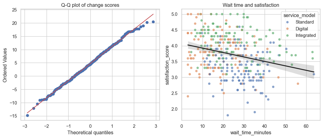
fig, axes = plt.subplots(1, 2, figsize=(11, 4.8))
stats.probplot(df["change_score"].dropna(), plot=axes[0])
axes[0].set_title("Q-Q plot of change scores")
sns.scatterplot(data=df, x="wait_time_minutes", y="satisfaction_score", hue="service_model", alpha=.65, ax=axes[1])
sns.regplot(data=df, x="wait_time_minutes", y="satisfaction_score", scatter=False, color="#222", ax=axes[1])
axes[1].set_title("Wait time and satisfaction")
plt.tight_layout()
plt.show()

Figure 2: A Q-Q diagnostic for change scores and the observed wait-time–satisfaction relationship.

Do not reject a method automatically because a large-sample normality test is significant. Combine design knowledge, graphical evidence, sample size, robustness, and sensitivity analyses.

Step 7: Test a Meaningful Benchmark — One-Sample t-Test

change = df["change_score"].dropna()
h1 = stats.ttest_1samp(change, popmean=3)
one_sided_p = h1.pvalue / 2 if h1.statistic > 0 else 1 - h1.pvalue / 2
estimate = change.mean() - 3
effect_size = estimate / change.std(ddof=1)
h1.statistic, one_sided_p, estimate, effect_size

(np.float64(5.003356552190933),
 np.float64(4.457311316749432e-07),
 np.float64(1.7121813031161466),
 np.float64(0.266301798953073))

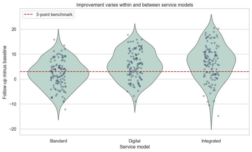
Decision rule: reject H0 when the prespecified one-sided p-value is below 0.05. Then interpret how far the mean lies above the benchmark and whether that excess is practically meaningful.

Step 8: Compare Independent Groups — Welch t-Test

integrated = df.loc[df["service_model"].eq("Integrated"), "change_score"].dropna()
standard = df.loc[df["service_model"].eq("Standard"), "change_score"].dropna()
h2 = stats.ttest_ind(integrated, standard, equal_var=False)
mean_difference = integrated.mean() - standard.mean()
pooled_sd = np.sqrt(((len(integrated)-1)*integrated.var(ddof=1) + (len(standard)-1)*standard.var(ddof=1)) / (len(integrated)+len(standard)-2))
cohens_d = mean_difference / pooled_sd
h2, mean_difference, cohens_d

(TtestResult(statistic=np.float64(5.5062088376419345), pvalue=np.float64(9.944608245509428e-08), df=np.float64(225.60662309271652)),
 np.float64(4.517539026629936),
 np.float64(0.7109550372224813))

Welch’s test is the default here because it does not require equal group variances. A statistically detectable difference is not automatically large, useful, or causal.

Step 9: Compare Repeated Measurements — Paired t-Test

paired = df[["baseline_score", "followup_score"]].dropna()
h3 = stats.ttest_rel(paired["followup_score"], paired["baseline_score"])
paired_change = paired["followup_score"] - paired["baseline_score"]
paired_d = paired_change.mean() / paired_change.std(ddof=1)
h3, paired_change.mean(), paired_d, len(paired)

(TtestResult(statistic=np.float64(13.769992205351423), pvalue=np.float64(8.24702963989523e-35), df=np.int64(352)),
 np.float64(4.712181303116147),
 np.float64(0.7329027339155224),
 353)

The pairing is essential: baseline and follow-up values belong to the same person. An independent t-test would discard that structure and answer the wrong question.

Step 10: Compare Three Groups — ANOVA

groups = [g["change_score"].dropna() for _, g in df.groupby("service_model")]
h4 = stats.f_oneway(*groups)
grand_mean = df["change_score"].mean()
ss_between = sum(len(g) * (g.mean() - grand_mean)**2 for g in groups)
ss_total = ((df["change_score"] - grand_mean)**2).sum()
eta_squared = ss_between / ss_total
h4, eta_squared

(F_onewayResult(statistic=np.float64(17.378972590583246), pvalue=np.float64(6.369103981488866e-08)),
 np.float64(0.09033717332282878))

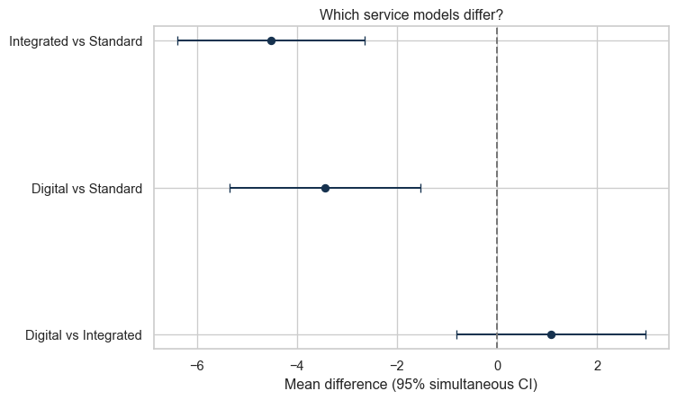
ANOVA answers whether at least one population mean differs. It does not identify which pairs differ, so a significant omnibus result must be followed by planned or multiplicity-controlled comparisons.

Step 11: Locate Differences — Tukey HSD

tukey = pairwise_tukeyhsd(
    endog=df.loc[df["change_score"].notna(), "change_score"],
    groups=df.loc[df["change_score"].notna(), "service_model"],
    alpha=ALPHA,
)
tukey_table = pd.DataFrame(tukey._results_table.data[1:], columns=tukey._results_table.data[0])
tukey_table

	group1	group2	meandiff	p-adj	lower	upper	reject
0	Digital	Integrated	1.0820	0.3680	-0.8031	2.9670	False
1	Digital	Standard	-3.4356	0.0001	-5.3362	-1.5349	True
2	Integrated	Standard	-4.5175	0.0000	-6.3943	-2.6408	True

tukey_plot = tukey_table.copy()
tukey_plot["comparison"] = tukey_plot["group1"].astype(str) + " vs " + tukey_plot["group2"].astype(str)
y = np.arange(len(tukey_plot))
fig, ax = plt.subplots(figsize=(8, 4.8))
ax.errorbar(tukey_plot["meandiff"], y, xerr=[tukey_plot["meandiff"]-tukey_plot["lower"], tukey_plot["upper"]-tukey_plot["meandiff"]], fmt="o", capsize=4, color="#16324f")
ax.axvline(0, color="#777", linestyle="--")
ax.set_yticks(y, tukey_plot["comparison"])
ax.set(xlabel="Mean difference (95% simultaneous CI)", title="Which service models differ?")
plt.tight_layout()
plt.show()

Figure 3: Tukey-adjusted pairwise mean differences with simultaneous 95% confidence intervals.

Step 12: Test Continuous Relationships — Pearson and Spearman

correlation_data = df[["wait_time_minutes", "satisfaction_score"]].dropna()
pearson = stats.pearsonr(correlation_data["wait_time_minutes"], correlation_data["satisfaction_score"])
age_satisfaction = df[["age", "satisfaction_score"]].dropna()
spearman = stats.spearmanr(age_satisfaction["age"], age_satisfaction["satisfaction_score"])
pearson, spearman

(PearsonRResult(statistic=np.float64(-0.26389263802754537), pvalue=np.float64(4.5523934529589285e-07)),
 SignificanceResult(statistic=np.float64(-0.03712241491653051), pvalue=np.float64(0.48940578089574993)))

Pearson tests the linear wait-time relationship. Spearman tests a separate monotonic age-satisfaction question and illustrates a defensible fail to reject H0 decision. That decision is insufficient evidence of a relationship, not proof of no relationship. Neither correlation establishes causality.

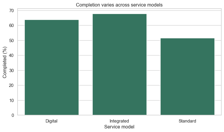
Step 13: Test Categorical Association — Chi-Square

observed = pd.crosstab(df["service_model"], df["completed_program"])
chi_square = stats.chi2_contingency(observed)
expected = pd.DataFrame(chi_square.expected_freq, index=observed.index, columns=observed.columns)
cramers_v = np.sqrt(chi_square.statistic / (observed.to_numpy().sum() * min(np.array(observed.shape)-1)))
observed, expected.round(2), chi_square, cramers_v

(completed_program  No  Yes
 service_model             
 Digital            42   74
 Integrated         40   84
 Standard           58   62,
 completed_program     No    Yes
 service_model                  
 Digital            45.11  70.89
 Integrated         48.22  75.78
 Standard           46.67  73.33,
 Chi2ContingencyResult(statistic=np.float64(7.149086286349914), pvalue=np.float64(0.028028227736802584), dof=2, expected_freq=array([[45.11111111, 70.88888889],
        [48.22222222, 75.77777778],
        [46.66666667, 73.33333333]])),
 np.float64(0.14092044925289818))

completion = pd.crosstab(df["service_model"], df["completed_program"], normalize="index").mul(100).reset_index()
fig, ax = plt.subplots(figsize=(8, 4.8))
sns.barplot(data=completion, x="service_model", y="Yes", color="#2a7f62", ax=ax)
ax.set(xlabel="Service model", ylabel="Completed (%)", title="Completion varies across service models")
plt.tight_layout()
plt.show()

Figure 4: Program-completion percentages by service model.

Step 14: Ask Whether Conclusions Survive Alternative Methods

mann_whitney = stats.mannwhitneyu(integrated, standard, alternative="two-sided")
wilcoxon = stats.wilcoxon(paired["followup_score"], paired["baseline_score"], alternative="two-sided")
kruskal = stats.kruskal(*groups)
mann_whitney, wilcoxon, kruskal

(MannwhitneyuResult(statistic=np.float64(9867.5), pvalue=np.float64(1.5083294351870063e-07)),
 WilcoxonResult(statistic=np.float64(9531.5), pvalue=np.float64(1.1073226595720851e-29)),
 KruskalResult(statistic=np.float64(31.832654684182707), pvalue=np.float64(1.2235644862257207e-07)))

Non-parametric tests answer related but not identical questions. Use them as sensitivity evidence, not as automatic replacements selected only because a normality p-value crossed 0.05.

Step 15: Control the Family of Hypotheses

raw_p_values = np.array([
    one_sided_p, h2.pvalue, h3.pvalue, h4.pvalue,
    pearson.pvalue, spearman.pvalue, chi_square.pvalue,
])
reject, adjusted_p, _, _ = multipletests(raw_p_values, alpha=ALPHA, method="holm")
hypothesis_ids = ["H1", "H2", "H3", "H4", "H5", "H6", "H7"]
pd.DataFrame({
    "test_id": hypothesis_ids,
    "raw_p_value": raw_p_values,
    "holm_adjusted_p_value": adjusted_p,
    "holm_decision": np.where(reject, "Reject H0", "Fail to reject H0"),
})

	test_id	raw_p_value	holm_adjusted_p_value	holm_decision
0	H1	4.457311e-07	1.782925e-06	Reject H0
1	H2	9.944608e-08	4.972304e-07	Reject H0
2	H3	8.247030e-35	5.772921e-34	Reject H0
3	H4	6.369104e-08	3.821462e-07	Reject H0
4	H5	4.552393e-07	1.782925e-06	Reject H0
5	H6	4.894058e-01	4.894058e-01	Fail to reject H0
6	H7	2.802823e-02	5.605646e-02	Fail to reject H0

Multiplicity correction protects against accumulating false-positive risk. It does not rescue an unfocused analysis plan; prespecify primary and supporting questions whenever possible.

Step 16: Build the Hypothesis Decision Register

For each hypothesis, record:

• the research question and estimand;
• H0 and H1;
• method and justification;
• relevant assumptions;
• sample size, estimate, and 95% confidence interval;
• effect size;
• raw and adjusted p-values;
• Reject H0 or Fail to reject H0;
• plain-language interpretation;
• practical importance; and
• limitations and unsupported claims.

The reference workflow exports results/tables/hypothesis-decision-register.csv. Treat this as the bridge from test output to accountable insight.

Step 17: Transform the Evidence into a CDI Insight Brief

Central question: Which service model produces the strongest outcomes, for whom, and how confidently can we defend that conclusion?

Key findings: State the most decision-relevant results, not every p-value.

Supporting evidence: Combine estimates, intervals, effect sizes, post-hoc contrasts, categorical results, and sensitivity checks.

Practical importance: Explain whether detected differences are large enough to matter.

Consistent or conflicting evidence: Identify where methods agree and where they do not.

Uncertainty and limitations: Address missingness, observational allocation, region composition, multiplicity, and measurement limitations.

Recommended action: Propose a proportionate next step supported by the evidence.

Claims not supported: Explicitly state what the analysis cannot establish.

A defensible conclusion might prioritize investigation of Integrated service features while improving Standard delivery, yet still recommend prospective confirmation before claiming the service model caused better outcomes.

Step 18: Complete an Independent Challenge

Choose one extension:

• test whether outcomes differ by region and consider whether region may confound service comparisons;
• examine whether the service-model effect differs across age groups;
• evaluate whether missing follow-up scores could change the conclusion; or
• define a new primary outcome and build a fresh decision-register entry.

Your extension must use the same CDI reasoning pattern and end with a bounded, evidence-supported insight.

Common Mistakes to Avoid

• choosing a test before defining the question and design;
• treating p < 0.05 as proof of importance or causality;
• saying “accept H0” after a non-significant result;
• running independent tests on paired observations;
• interpreting ANOVA as proof that every group differs;
• reporting only p-values without estimates, intervals, and effects;
• using assumption tests mechanically without inspecting plots and design;
• conducting many unplanned tests without multiplicity control;
• converting association into causal language; and
• hiding uncertainty or evidence that conflicts with the preferred narrative.

Completion Checklist

• Dataset generated and validated
• Missingness and study design documented
• Seven hypotheses defined before interpretation
• One-sample, independent, and paired t-tests completed
• ANOVA and Tukey HSD completed
• Pearson and Spearman correlations compared
• Chi-square assumptions and effect size evaluated
• Non-parametric sensitivity analyses completed
• Holm-adjusted decisions recorded
• Four figures interpreted
• Hypothesis decision register completed
• Independent challenge completed
• CDI Insight Brief written with limitations and unsupported claims

Final Reflection

The statistical test is not the product. The product is a clear, defensible insight that respects study design, uncertainty, practical importance, alternative explanations, and the limits of the evidence.

© Complex Data Insights | CDI Practicals

Hands-on exercises and step-by-step tools